[WIP] The Algorithm Design Manual - Notes

Pet Peeve: The author sometimes skips steps without an explaination (like the integer truncation in "stop and think: incremental correctness"). Some examples are hard to follow for an international student (like understanding the lottery system in "war story: pschic modeling").

Chapter 1 — Introduction to Algorithm Design

1. An algorithmic problem is specified by describing the complete set of instances it must work on and of its output after running on one of these instances.

2. An algorithm is a procedure that takes any of the possible input instances and transforms it to the desired output.

3. There is a distinction between a general problem and an instance of a problem. E.g:

   Problem: Sorting
   Input: A sequence of n keys a₁,...,a_n.
   Output: The permutation (reordering) of the input sequence such that: a′₁ ≤ a′₂ ≤ ··· ≤ a′_n−1 ≤ a′_n.
   Instance of sorting problem: { Mike, Bob, Sally}; { 154, 245 }

4. Insertion sort is an algorithm to the sorting problem: English description:

   Start with a single element (thus forming a trivially sorted list) and then incrementally inserts the remaining elements so that the list stays sorted.

   Pseudocode:

   Copycopy code to clipboard
   1array = input sequence
   2n = array size
   3i = 0
   4
   5while i < n
   6   j = i
   7   while j > 0 AND array[j] < array[j - 1]
   8       swap element at `j` with element at `j - 1` in array
   9       decrement j by 1
   10   increment i by 1

   Code:

   Copycopy code to clipboard
   1insertion_sort(item s[], int n)
   2 {
   3   int i,j; /* counters */
   4   for (i=0; i<n; i++) {
   5     j=i;
   6     
   7     while ((j>0) && (s[j] < s[j-1])) {
   8       swap(&s[j],&s[j-1]);
   9       j = j-1;
   10     }
   11   }
   12 }

   An animation of the logical flow of this algorithm on a particular instance (the letters in the word “INSERTIONSORT”)

5. There is a fundamental difference between algorithms, which always produce a correct result, and heuristics, which may usually do a good job but without providing any guarantee.

6. Three desirable properties for a good algorithm:

   • correct
   • efficient
   • easy to implement

7. Correct algorithms usually come with a proof of correctness, which is an explanation of why we know that the algorithm must take every instance of the problem to the desired result.

Robot Tour Optimization

Problem: Robot Tour Optimization (aka: Traveling Salesman Problem [TSP]).
Input: A set S of n points in the plane.
Output: What is the shortest cycle tour that visits each point in the set S?

Nearest-neighbor heuristic

1. English Description:

   Starting from some point p0, we walk first to its nearest neighbor p1 From p1, we walk to its nearest unvisited neighbor. Repeat this process until we run out of unvisited points After which we return to p0 to close off the tour.

2. Pseudocode:

   Copycopy code to clipboard
   1NearestNeighbor(P)
   2   Pick and visit an initial point p₀ from P
   3   p = p₀
   4   i = 0
   5   
   6   While there are still unvisited points
   7       i = i + 1
   8       Select pᵢ to be the closest unvisited point to pᵢ₋₁
   9       Visit pᵢ
   10   Return to p₀ from pₙ₋₁

3. Pros:
   • Easy to understand & implement
   • Reasonably efficient
4. Cons: It's wrong — It always finds a tour, but it doesn’t necessarily find the shortest possible tour. E.g: A bad instance for the nearest-neighbor heuristic (top) & the optimal solution (bottom):

Closest-pair heuristic

1. English description:

   Repeatedly connect the closest pair of endpoints whose connection will not create a problem, such as premature termination of the cycle. Each vertex begins as its own single vertex chain. After merging everything together, we will end up with a single chain containing all the points in it. Connecting the final two endpoints gives us a cycle. At any step during the execution of this closest-pair heuristic, we will have a set of single vertices and vertex-disjoint chains available to merge.

2. Pseudocode:

Reasoning about Correctness

1. We need tools to distinguish correct algorithms from incorrect ones, the primary one of which is called a proof.
2. A proper mathematical proof consists of several parts:
   • A clear, precise statement of what you are trying to prove.
   • A set of assumptions of things that are taken to be true, and hence can be used as part of the proof.
   • A chain of reasoning that takes you from these assumptions to the statement you are trying to prove.
   • A little square (■) or QED at the bottom to denote that you have finished, representing the Latin phrase for "thus it is demonstrated."
3. A proof is indeed a demonstration. Proofs are useful only when they are honest, crisp arguments that explain why an algorithm satisfies a non-trivial correctness property.

Problems and Properties

1. It is impossible to prove the correctness of an algorithm for a fuzzily-stated problem.
2. Problem specifications have two parts:

   Copycopy code to clipboard
   1* The set of allowed input instances.
   2* The required properties of the algorithm's

   output.
3. An important technique in algorithm design is to narrow the set of allowable instances until there is a correct and efficient algorithm. For example, we can restrict a graph problem from general graphs down to trees, or a geometric problem from two dimensions down to one.
4. There are two common traps when specifying the output requirements of a problem:

   Copycopy code to clipboard
   1* Asking an ill-defined question. E.g: Asking for the best route between two places on a map is a silly question, unless you define what best means.
   2* Creating compound goals. E.g: A goal like find the shortest route from **a** to **b** that doesn't use more than twice as many turns as necessary is perfectly well defined, but complicated to reason about and solve.

Expressing Algorithms

1. The heart of any algorithm is an idea. If your idea is not clearly revealed when you express an algorithm, then you are using too low-level a notation to describe it.
2. The three most common forms of algorithmic notation are
   • English
   • Pseudocode (a programming language that never complains about syntax errors)
   • A real programming language.
3. All three methods are useful because there is a natural tradeoff between greater ease of expression and precision.

Demonstrating Incorrectness

1. The best way to prove that an algorithm is incorrect is to produce a counter example, i.e: an instance on which it yields an incorrect answer.
2. Good counterexamples have two important properties:
   • Verifiability: To demonstrate that a particular instance is a counterexample to a particular algorithm, you must be able to:
     • calculate what answer your algorithm will give in this instance, and
     • display a better answer so as to prove that the algorithm didn't find it.
   • Simplicity - Good counter-examples have all unnecessary details stripped away. They make clear exactly why the proposed algorithm fails. Simplicity is important because you must be able to hold the given instance in your head in order to reason about it.

Induction and Recursion

1. Recursion is mathematical induction in action. In both, we have general and boundary conditions, with the general condition breaking the problem into smaller and smaller pieces. The initial or boundary condition terminates the recursion.
2. The simplest and most common form of mathematical induction infers that a statement involving a natural number n (that is, an integer n ≥ 0) holds for all values of n. The proof consists of two steps:
   • The initial or base case: prove that the statement holds for a fixed natural number (usually 0 or 1).
   • The induction/inductive step: assume that the statement holds for some arbitrary natural number n = k, and prove that the statement holds for n = k + 1.
3. The hypothesis in the inductive step, that the statement holds for n = k, is called the induction/inductive hypothesis. You're doing a thought experiment of what would happen if it was true for n = k. It might be clearer to use the phrase "suppose true when n = k" rather than "assume true when n = k" to emphasise this.
4. To prove the inductive step, one assumes the induction hypothesis for n = k and then uses this assumption to prove that the statement holds for n = k + 1. We try to manipulate the statement for n = k + 1 so that it involves the case for n = k (which we assumed to be true).

Inductive proof for Insertion sort

1. The basis case consists of a single element, and by definition a one-element array is completely sorted.
2. We assume that the first n - 1 elements of array A are completely sorted after n - 1 iterations of insertion sort.
3. To insert one last element x to A, we find where it goes, namely the unique spot between the biggest element less than or equal to x and the smallest element greater than x. This is done by moving all the greater elements back by one position, creating room for x in the desired location. ■

Modeling the Problem

1. Modeling is the art of formulating your application in terms of precisely described, well-understood problems.
2. Proper modeling is the key to applying algorithmic design techniques to real-world problems — it can eliminate the need to design an algorithm, by relating your application to what has been done before.
3. Real-world applications involve real-world objects — like a system to route traffic in a network or find the best way to schedule classrooms in a university.
4. Most algorithms, however, are designed to work on rigorously defined abstract structures such as permutations, graphs, and sets.
5. To exploit the algorithms literature, you must learn to describe your problem abstractly, in terms of procedures on such fundamental structures.
6. The act of modeling reduces your application to one of a small number of existing problems and structures. Such a process is inherently constraining, and certain details might not fit easily into the given target problem.
7. Certain problems can be modeled in several different ways, some much better than others.
8. Modeling is only the first step in designing an algorithm for a problem. Be alert for how the details of your applications differ from a candidate model, but don't be too quick to say that your problem is unique and special.

Combinatorial Objects

1. Permutations are arrangements, or orderings, of items. E.g: {1,4,3,2} and {4,3,2,1} are two distinct permutations of the same set of four integers.
2. Subsets represent selections from a set of items. E.g: {1,3,4} and {2} are two distinct subsets of the first four integers. Order does not matter in subsets the way it does with permutations.
3. Trees represent hierarchical relationships between items.
4. Graphs represent relationships between arbitrary pairs of objects.
5. Points define locations in some geometric space.
6. Polygons define regions in some geometric spaces.
7. Strings represent sequences of characters, or patterns.

Recursive Objects

Learning to think recursively is learning to look for big things that are made from smaller things of exactly the same type as the big thing.
If you think of houses as sets of rooms, then adding or deleting a room still leaves a house behind.

1. Permutations: Delete the first element of a permutation of n things {1, ..., n} and you get a permutation of the remaining n-1 things. Basis case: {}
2. Subsets: Every subset of {1, ..., n} contains a subset of (1, ..., n - 1) obtained by deleting element n. Basis case: {}
3. Trees: Delete the root of a tree and you get a collection of smaller trees. Delete any leaf of a tree and you get a slightly smaller tree. Basis case: 1 vertex.
4. Graphs: Delete any vertex from a graph, and you get a smaller graph. Now divide the vertices of a graph into two groups, left and right. Cut through all edges that span from left to right, and you get two smaller graphs, and a bunch of broken edges. Basis case: 1 vertex.
5. Point sets: Take a cloud of points, and separate them into two groups by drawing a line. Now you have two smaller clouds of points. Basis case: 1 point.
6. Polygons: Inserting any internal chord between two non-adjacent vertices of a simple polygon cuts it into two smaller polygons. Basis case: triangle.
7. Strings: Delete the first character from a string, and you get a shorter string. Basis case: empty string.

Recursive descriptions of objects require both decomposition rules and basis cases, namely the specification of the smallest and simplest objects where the decomposition stops.

Proof by Contradiction

1. The basic scheme of a contradiction argument is as follows:
   • Assume that the hypothesis (the statement you want to prove) is false.
   • Develop some logical consequences of this assumption.
   • Show that one consequence is demonstrably false, thereby showing that the assumption is incorrect and the hypothesis is true.
2. The classic contradiction argument is Euclid's proof that there are an infinite number of prime numbers:
   • The negation of the claim would be that there are only a finite number of primes, say m, which can be listed as p₁,..., pₘ. So let's assume this is the case and work with it.
   • Prime numbers have particular properties with respect to division. Suppose we construct the integer formed as the product of "all" of the listed primes: [ N = \prod{i = 1}^{m} p{i} ]
   • This integer N has the property that it is divisible by each and every one of the known primes, because of how it was built.
   • But consider the integer N + 1. It can't be divisible by p₁ = 2, because N is.
   • The same is true for p₂ = 3 and every other listed prime. Since a +1 can’t be evenly split by any of the prime numbers because they are bigger.
   • Since N + 1 doesn't have any non-trivial factor, this means it must be prime.
   • But you asserted that there are exactly m prime numbers, none of which are N + 1, because N + 1 > m.
   • This assertion is false, so there cannot be a bounded number of primes.
3. For a contradiction argument to be convincing, the final consequence must be clearly, ridiculously false.

Estimation

1. Principled guessing is called estimation.
2. Estimation problems are best solved through some kind of logical reasoning process, typically a mix of principled calculations and analogies.
3. Principled calculations give the answer as a function of quantities that either you already know, can look up on Google, or feel confident enough to guess.
4. Analogies reference your past experiences, recalling those that seem similar to some aspect of the problem at hand.

Exercises

Finding counter examples

1. Show that a + b can be less than min(a, b).

   When:
      a and b < 0 (i.e: negative)
      a <= b
   Then:
      min(a, b) = a
   a + b < a
   Example:
      min(-6, -5) = -6
   -6 + -5 = -6 -5 = -11
   -11 < -6

2. Show that a × b can be less than min(a, b).

   When:
      a < 0 (i.e: negative)
      b > 0 (i.e: positive)
   Then:
      min(a, b) = a
   a * b < a
   Example:
      min(-3, 4) = -3
   -3 * 4 = -12
   -12 < -3

3. Design/draw a road network with two points a and b such that the fastest route between a and b is not the shortest route.

   Copycopy code to clipboard
   1a──────c──────b
   2│             │
   3│             │
   4└────d────────┘
   5
   6Route `acb` have a toll gate, is in development and have a speed limit.
   7Route `adb` is longer, but has none of these impediment.
   8
   9Route `adb` will be faster than the shorter `acb` route.

4. Design/draw a road network with two points a and b such that the shortest route between a and b is not the route with the fewest turns.

   Copycopy code to clipboard
   1a────┐   ┌────b
   2│    └─c─┘    │
   3│             │
   4└──────d──────┘
   5
   6Route `acb` is the shortest but has 4 turns.
   7Route `adb` is the longest and has only 2 turns.

Induction

1. Prove that $\sum_{i = 1}^{n} i = \frac{n(n + 1)}{2}$ for n ≥ 0, by induction.

Chapter 2: Algorithm Analysis

The analysis of algorithms is the process of finding the computational complexity of algorithms.

For an ordered list of size $n$ ($33$ in the example above), binary search takes at most $\log_2 n$ check steps ($5$ steps in the example above); while linear search takes at most $n$ check steps ($28$ steps in the example above).

🏋️‍♀️ Computational complexity

The computational complexity or simply complexity of an algorithm is the amount of resources required to run it.

Common types of resources include:

1. ⏳ Time — Time complexity is the computational complexity that describes the amount of computer time it takes to run an algorithm. When "complexity" is used without qualification, this generally means time complexity.
2. 🫙 Memory — Space complexity is the computational complexity that describes the amount of memory it takes to run an algorithm.
3. 🎙️ Communication — The necessary amount of communication between executing parties in a distributed algorithm.

The computational complexity of an algorithm can be measured only when given a model of computation.

💻 The RAM model of computation

The most commonly used model of computation is the Random Access Machine (RAM) which is a hypothetical computation model where:

• Each simple operation (like +, *, -, =, if, call, etc) takes exactly unit-time (i.e. 1 step).
• Each complex operation (like loops and subroutines) is the composition of simple operations. The time it takes to run through a loop or execute a subprogram depends upon the number of loop iterations or the specific nature of the subprogram.
• Each memory access takes exactly unit-time (i.e. 1 step), regardless of data location (cache or disk). There is also unlimited memory.

The RAM is a simple model of how computers perform. It allows the analysis of algorithms in a machine-independent way by assuming that simple operations take a constant amount of time on a given computer and change only by a constant factor when run on a different computer.

It doesn’t capture the full complexity of real computers (e.g. multiplying two numbers takes more time than adding two numbers on most processors). However, the RAM is still an excellent model for understanding how an algorithm will perform on a real computer.

A model is a simplification or approximation of reality and hence will not reflect all of reality. […] "all models are wrong, but some are useful." — Model Selection and Multimodel Inference

🏭 Computational complexity functions

Under the RAM model, we measure the computational complexity by counting the number of simple operations (also called steps) an algorithm takes on a given problem instance.

As the amount of resources required to run an algorithm generally varies with the size of the input, the complexity is typically expressed as a function $n \rightarrow f(n)$, where $n$ is the size of the input and $f(n)$ is the computational complexity.

Aside: We can also use any other characteristic of the input influencing the computational complexity.

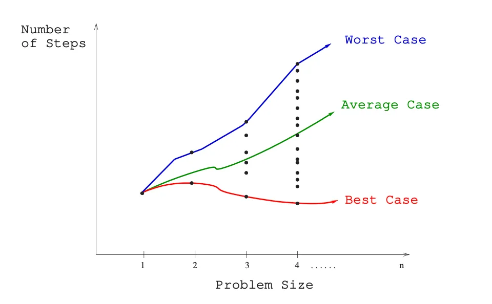
However, the complexity of an algorithm may vary dramatically for different inputs of the same size. Therefore, three complexity functions are commonly used:

1. 🔵 Worst-case complexity: is the maximum of the complexity over all inputs of size $n$.
   • It expresses the resources used by an algorithm at most.
   • e.g. the worst-case time complexity for a simple linear search on a list is $n$ and occurs when the desired element is the last element of the list or is not in the list.
   • Worst-case analysis gives a safe analysis (the worst case is never underestimated), but one which can be overly pessimistic, since there may be no (realistic) input that would take this many steps.
   • Generally, when "complexity" is used without being further specified, this is the worst-case computational complexity that is considered.
2. 🟢 Average-case complexity: is the average of the complexity over all inputs of size $n$.
   • It expresses the resources used by an algorithm on average.
   • Average-case analysis requires a notion of an "average" input to an algorithm, which leads to the problem of devising a probability distribution over inputs.
   • e.g. the average-case time complexity for a simple linear search on a list is $n/2$ assuming the value searched for is in the list and each list element is equally likely to be the value searched for.
   • Con: Determining what typical input means is difficult and average case analysis tends to be more difficult.
3. 🔴 Best-case complexity: is the minimum of the complexity over all inputs of size $n$.
   • It expresses the resources used by an algorithm at least.
   • e.g. the best case time complexity for a simple linear search on a list is $1$ and occurs when the desired element is the first element of the list.
   • Con: It's unlikely to happen in practice.

📈 Big oh notation

There are three problems with the complexity functions above:

1. The exact computational complexity functions for any algorithm are liable to be complicated because they tend to have lots of up-and-down bumps.
2. In addition, these exact values provide little practical application, as any change of computer or model of computation would change the complexity somewhat.
3. Moreover, the resource use is not critical for small values of $n$.

Complexity theory seeks to quantify the intrinsic time requirements of algorithms (independent of any external factors), that is, the basic time constraints an algorithm would place on any computer .

For these reasons, one generally focuses on the behavior of the complexity for large $n$, that is on its asymptotic behavior when $n$ tends to infinity. Therefore, the complexity is generally expressed by using big O notation.

Big O notation is a mathematical notation that describes the limiting behavior of a function when the argument tends towards infinity. The formal definition of the big O notations are:

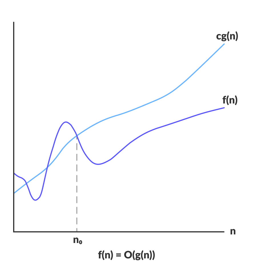
1. Big O (Upper bound)

Notation: $f(n) = O(g(n))$

Meaning: There exists some constant $c$ such that $|f(n)| \leq c \cdot |g(x)|$ for large enough $n$ (i.e. for all $n \geq n_0$, for some constant $n_0$).

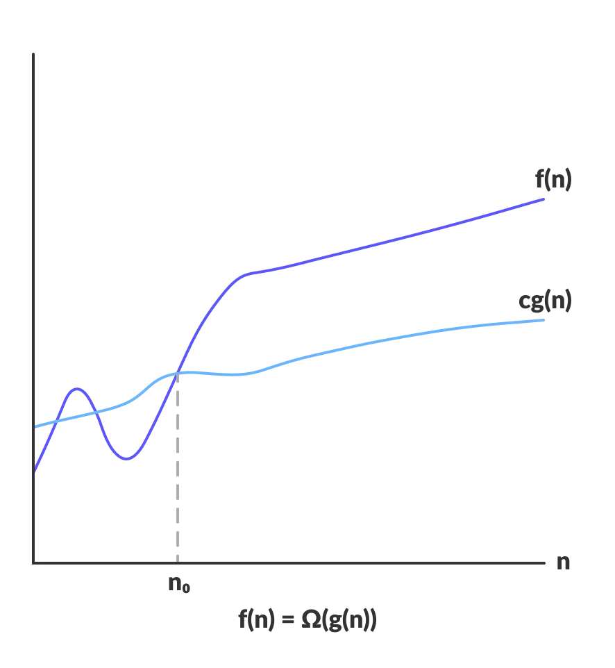
2. Big Omega (Lower bound)

Notation: $f(n) = \Omega(g(n))$

Meaning: Means there exists some constant $c$ such that $|f(n)| \geq c \cdot |g(x)|$ for large enough $n$ (i.e. for all $n \geq n_0$, for some constant $n_0$).

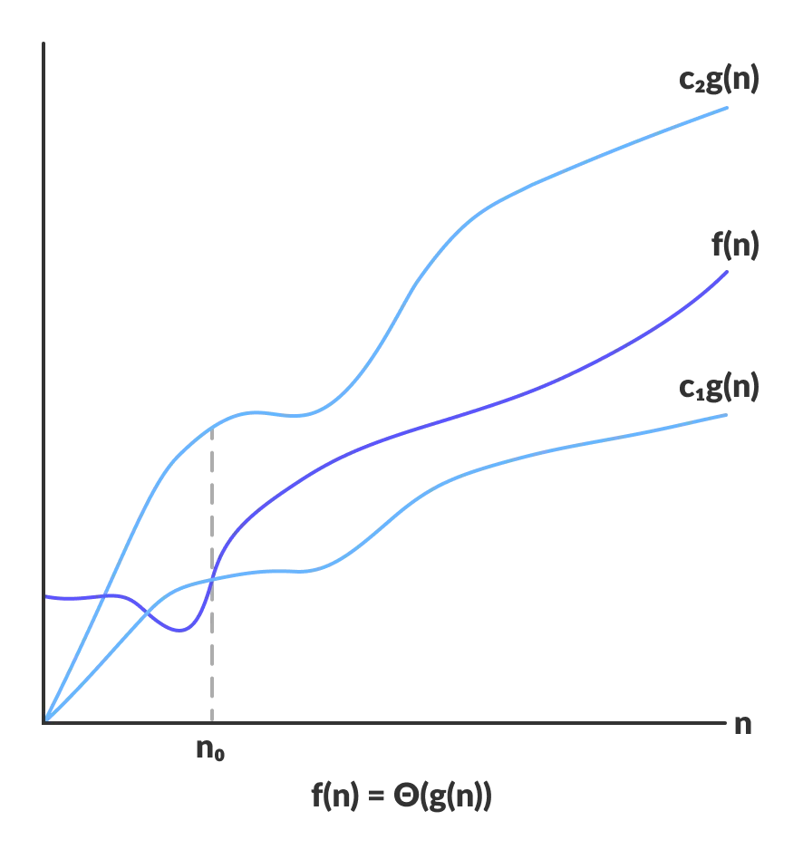
3. Big Theta (Tight bound [upper & lower bound])

Notation: $f(n) = \Theta(g(n))$

Meaning: Means there exists some constants $c_1$ and $c_2$ such that $|f(n)| \leq c_1 \cdot |g(x)|$ and $|f(n)| \geq c_2 \cdot |g(x)|$ for large enough $n$ (i.e. for all $n \geq n_0$, for some constant $n_0$).

🙅‍♂️ Misconception: Conflating Big-O with complexity functions

The best/average/worst-case computational complexity is a function of the size of the input for a certain algorithm.

The $O$, $\Omega$, and $\Theta$ notations are used to describe the relationship between two functions.

Hence, each best/average/worst case computational complexity function has its corresponding $O$, $\Omega$, and $\Theta$ notation.

Conflating the big O notations with the computational complexity functions likely stems from the fact that in everyday use, “the big O of the worst-case computational complexity function” is used interchangeably with just “big O”, “time complexity”, “complexity”, etc.

🙈 Abuse of notation

There are two accepted abuses of notation in the computer science industry:

1. Abuse of the equal sign: Technically, the appropriate notation is $f(n) \in O(g(n))$, because the equal sign does not imply symmetry.

2. Abuse of the Big O notation: The big O notation is often used to describe an asymptotic tight bound where using big Theta $\Theta$ notation would be more factually appropriate. Big O notation provides an upper bound, but it doesn't necessarily provide a tight upper bound. For example, $2n^2 + 3n + 1$ is $O(n^2)$, but it is also $O(n^3)$, $O(n^4)$, etc. For contrast, the equation is only $\Theta(n^2)$.

Common Big O functions

The function $g(x)$ appearing within the $O(·)$ is typically chosen to be as simple as possible, omitting constant factors and lower-order terms.

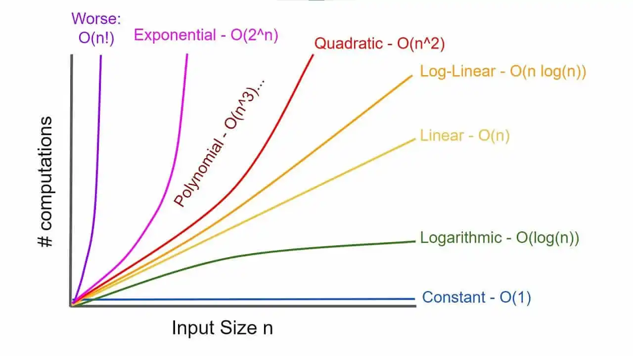
• Constant functions:

  • $f(n) = 1$
  • In the big picture, there is no dependence on the parameter $n$.
  • Such functions might measure the cost of adding two numbers or the growth realized by functions such as $f(n) = min(n, 100)$.

• Logarithmic functions:

  • $f(n) = \log_2 n$
  • Logarithmic time complexity shows up in algorithms such as binary search
  • Such functions grow quite slowly as $n$ gets big.

• Linear functions:

  • $f(n) = n$
  • Such functions measure the cost of looking at each item once (or twice, or ten times) in an $n$-element array, say to identify the biggest item, the smallest item, or compute the average value.

• Superlinear functions:

  • $f(n) = n \log_2 n$
  • This important class of functions arises in such algorithms as Quicksort and Mergesort.

• Quadratic functions:

  • $f(n) = n^2$
  • Such functions measure the cost of looking at most or all pairs of items in an $n$-element universe. This arises in algorithms such as insertion sort and selection sort.

• Cubic functions:

  • $f(n) = n^3$
  • Such functions enumerate through all triples of items in an $n$-element universe.

• Exponential functions:

  • $f(n) = c^n$ for a given constant $c > 1$
  • Functions like $2^n$ arise when enumerating all subsets of $n$ items.

• Factorial functions:

  • $f(n) = n!$
  • Functions like $n!$ arise when generating all permutations or orderings of $n$ items.

Arithmetic operations with Big O notation

1. Addition:

   • If $f(n)$ is $O(g(n))$ and $h(n)$ is $O(k(n))$, then $f(n) + h(n)$ is $O(\max(g(n), k(n)))$.
   • This is because the dominant function among $g(n)$ and $k(n)$ will dictate the overall growth rate.

2. Multiplication by a constant:

   • If $f(n)$ is $O(g(n))$, then $c \cdot f(n)$ is $O(g(n))$ for any constant $c > 0$.
   • This is because multiplying a function by a constant simply scales the function but does not change its growth rate.

3. Multiplication:

   • If $f(n)$ is $O(g(n))$ and $h(n)$ is $O(k(n))$, then $f(n) \cdot h(n)$ is $O(g(n) \cdot k(n))$.
   • TODO: This is because in the worst case, the product of the dominant terms will determine the overall growth rate.

4. Division:

   • If $f(n)$ is $O(g(n))$ and $g(n)$ is bounded away from zero, then $f(n) / g(n)$ is $O(1)$.
   • This is because, in the limit, the ratio converges to a constant.

5. Transitivity:

   • If $f(n)$ is $O(g(n))$ and $g(n)$ is $O(h(n))$, then $f(n)$ is $O(h(n))$.
   • This property allows for chaining comparisons of functions.

Reasoning about an algorithm's efficiency

1. Selection sort

Copycopy code to clipboard
1// Selection sort repeatedly identifies the smallest remaining unsorted element
2// and puts it at the end of the sorted portion of the array.
3void selectionSort(int arr[], int n) {
4    int i, j, minimum_element_index;
5
6    // One by one move the boundary of the unsorted subarray
7    for (i = 0; i < n; i++) {
8
9        // Find the minimum element in the unsorted array
10        minimum_element_index = i;  // Assume the current element is the minimum
11        
12        for (j = i + 1; j < n; j++) {
13            // If we find a smaller element, update the minimum_element_index
14            if (arr[j] < arr[minimum_element_index]) {
15                minimum_element_index = j;
16            }
17        }
18
19        // Swap the found minimum element with the first element
20        swap(&arr[minimum_element_index], &arr[i]);
21    }
22}

Analysis of the selection sort algorithm:

1. The outer loop goes around $n$ times.
2. The nested inner loop goes around $n - (i + 1)$ times, where $i$ is the index of the outer loop.
3. The exact number of times the if statement is executed is:$$T(n) = \sum_{i=0}^{n-1} \sum_{j=i+1}^{n-1} 1$$
   • To calculate the inner summation, we multiply the number of terms by $1$.
   • The number of terms in a summation can be calculated by subtracting the lower limit from the upper limit of the summation and then adding 1.
   • This gives $(n - 1) - (i + 1) + 1$ which equals $n - i - 1$.
   • Hence, the original equation simplifies to:
   $$\sum_{i=0}^{n-1} n - i - 1$$
4. What the sum is doing is adding up the non-negative integers in decreasing order starting from $n - 1$:$$T(n) = (n - 1) + (n - 2) + (n - 3) + ... + 2 + 1 + 0$$
5. The formula for the sum of the first $n$ non-negative integers (also known as the sum of an arithmetic series) is given by:$$\sum_{i=0}^{n-1} i = \frac{n(n - 1)}{2}$$
6. Hence, we can simply the summation to:$$\sum_{i=0}^{n-1} n - i - 1 = \frac{n(n - 1)}{2}\\ = \frac{n^2 - n}{2}$$
7. Therefore the time complexity of selection sort is:
   • $O(n^2)$
   • $\Omega(n^2)$
   • $\Theta(n^2)$

Logarithms and their applications

A logarithm is an inverse exponential function:

Exponential functions grow at a fast rate while logarithmic growth at a slow rate. Logarithms arise in any process where things are repeatedly halved. e.g.

1. Logarithms and binary search:

   • Binary search is an example of an $O(log n)$ algorithm.
   • The size of the list is halved with each iteration of the algorithm.
   • Thus, only $20$ comparisons suffice to find an element in an array with 1 million elements.

2. Logarithms and trees:

   • A binary tree of height $1$ can have up to $2$ leaf nodes, while one of height $2$ can have up to $4$ leaves. The number of leaves doubles each time we increase the height by $1$.
   • To generalize to trees that have $d$ children, a tree of height $1$ can have up to $d$ leaf nodes, while one of height $2$ can have up to $d^2$ leaves. The number of leaves multiplies by $d$ each time we increase the height by $1$.
   • To account for $n$ leaves, $n = d^h$, which implies that $h = \log_d n$

3. Logarithms and bits:

   • There are $2$ bit patterns of length $1$ (i.e. 0 and 1), $4$ of length $2$ (i.e. 00, 11, 10, 01), and $8$ of length 3.
   • The number of bit patterns doubles with each increase in the number of bits.
   • Let $w$ represent number of bits and $n$ represent number of bit patterns. Then $2^w = n$ or $w = \log_2 n$.

Product property of logarithms

A direct consequence of the product property is the power property:

Since $c$ is a constant, this implies raising the logarithm’s argument to a power doesn't affect the growth rate:

Change of base property of logarithms

Changing the base of $\log_b (a)$ to base-c simply involves multiplying by $\log_c (b)$:

Since $c$ and $b$ are constants, this property implies that the base of a logarithm has no impact on the growth rate:

Aside: In practice, an asymptotically inefficient algorithm may be more efficient for small input sizes. This is particularly used in hybrid algorithms, like Timsort, which use an asymptotically efficient algorithm (here merge sort, with time complexity $n \log n$), but switch to an asymptotically inefficient algorithm (here insertion sort, with time complexity $n^2$) for small data, as the simpler algorithm is faster on small data.

Chapter 3: Data structures

1. A data type (or simply type) is a collection of data values, usually specified by:
   • A set of possible values,
   • A set of allowed operations on these values, and/or
   • A representation of these values as machine types.
2. An abstract data type (ADT) is a data type that does not specify the concrete representation of the data. They are defined by their behavior (semantics) from the point of view of a user of the data, specifically in terms of:
   • Possible values, and
   • Possible operations on data of this type.
3. The generic definition of data structure is anything that can hold your data in a structured way. ADT contrasts with data structures, which are concrete representations of data, and are the point of view of an implementer.
4. The distinction between ADTs and data structures lies in the POV / level of abstraction. Some important points:
   • User’s POV: An int in a programming language sense is a fixed-width data structure. An integer in a mathematical sense is an ADT. For most purposes the user can work with the abstraction rather than the concrete choice of representation, and can simply use the data as if the type were truly abstract.
   • Name overloading: An array is an ADT when viewed as a collection of items that can be accessed by an index. An array is a data structure when viewed as a collection of fixed sized items stored as contiguous blocks in memory.
   • ADT implementations: There are multiple implementations of an ADT. E.g: A list can be implemented as an array or a linked-list.
5. Data structures can be classified into:
   • Contiguous data structures: composed of single slabs of memory. E.g. arrays, matrices, heaps, hash tables, etc.
   • Linked data structures: composed of distinct chunks of memory bound together by pointers. E.g. linked-list, trees, graph adjacency lists, etc.

Arrays

1. Arrays are data structures of fixed-size elements stored contiguously such that each element can be efficiently located by its index.$$ElementAddress(i) = FirstElementAddress + (i \cdot ElementSize)$$
2. Advantages of arrays:
   • Constant-time access given the index: because the index of each element maps directly to a particular memory address.
   • Space efficiency: because no space is wasted with links, end-of-element information, or other per element metadata.
   • Memory locality: because the physical continuity between successive data access helps exploit the high-speed cache memory on modern computer architecture.
3. The primary disadvantage of arrays is that the number of elements (i.e. the array size) is fixed. The capacity needs to be specified at allocation.
4. Dynamic arrays overcome the fixed-size limitation of static arrays.
5. It does so by internally resizing when its capacity is exceeded:
   • Allocates a new bigger contiguous array.
   • Copy the content of the old array to the new array.
6. To avoid incurring the cost of resizing many times, dynamic arrays resize by a large amount, such as doubling in size.
7. Expanding the array by any constant proportion $a$ ensures that inserting $n$ elements takes $O(n)$ time overall, meaning that each insertion takes amortized $O(1)$ time. As $n$ elements are added, the capacities form a geometric progression.
8. The key idea of amortized analysis is to consider the worst-case cost of a sequence of operations on a data structure, rather than the worst-case individual cost of any particular operation.
9. The aggregate method is one of the methods for performing amortized analysis. In this method, the total cost of performing a sequence of $m$ operations on the data structure is divided by the number of operations $m$, yielding an average cost per operation, which is defined as the amortized cost.
10. The aggregate method of amortized analysis applied to dynamic arrays with doubling:

• $$t(i) = \begin{cases} 2^{k}+1 &\text{if } i = 2^{k} + 1\\ \end{cases}$$

• $t(i)$ defines the time it takes to perform the $i$-th addition.

• The first case of $t(i)$:

  • Defines the time taken when the array’s capacity is exceeded and has to doubled.
  • $k$ is a non-negative integer.
  • Because the array's capacity is doubled, this case happens when: $i = 2^{0} + 1$, $i = 2^{1} + 1$, ..., $i = 2^{n} + 1$.
  • The time taken is $2^{k}+1$ because:
    • $2^{k}$ elements has to be copied to the new array and
    • The $i$-th element has to be added into the new array. This represents the $+1$.

• The second case of $t(i)$:

  • Defines the time taken when the array capacity is not exceeded.
  • This is constant time because only a single addition is performed.

• e.g. Given a dynamic array initialized with a capacity of $1$:

  i	1	2	3	4	5	6	7	8	9	10
  $t(i)$	$1$	$2$	$3$	$1$	$5$	$1$	$1$	$1$	$9$	$1$
  Capacity	$1$	$2$	$4$	$4$	$8$	$8$	$8$	$8$	$16$	$16$

• $$Amortized \space cost = \frac{\sum_{i=1}^{n}t(i)}{n}$$

• e.g. Given $n = 4$:

  $$Amortized \space cost = \frac{\sum_{i=1}^{4}t(i)}{n}\\ = 1 + (2^0 + 1) + (2^1 + 1) + 1$$

• We see that in both cases of the function, there is a $+1$. So summation from $1$ to $n$ results in:

  $$\sum_{i=1}^{n}t(i) = n + \sum_{k=0}^{\log_2 (n - 1)}2^{k}$$

• The second operand represents the total cost of the copy operation that occurs on each resizing. For $n$ addition, this happens $\log_2 (n - 1) + 1$ times. e.g.

  n	1	2	3	4	5	6	7	8	9	10
  $\log_2 (n - 1)$		$0$	$1$	$1$	$2$	$2$	$2$	$2$	$3$	$3$
  $\sum_{k=0}^{\log_2 (n - 1)}2^{k}$		$1$	$3$	$3$	$7$	$7$	$7$	$7$	$15$	$15$

• The second operand is the partial sum of a geometric series, which has the formula:

  $$\sum_{k=0}^{n}x^{k} = \frac{x^{n+1} - 1}{x - 1}$$

• Applying the formula to the second operand:

  $$\sum_{k=0}^{\log_2 (n - 1)}2^{k} = \frac{2^{\log_2 (n - 1) + 1} - 1}{2 - 1}\\ = \frac{2^{\log_2 (n - 1) + 1} - 1}{1}\\ = 2^{\log_2 (n - 1) + 1} - 1\\ = 2^{\log_2 (n - 1)} \cdot 2^{1} - 1$$

• $\log_2 (n - 1)$ is the number to which $2$ must be raised to obtain $n - 1$. Raising that number then to $2$ results in $n - 1$. Hence, the last expression can be simplified to:

  $$= (n - 1) \cdot 2^{1} - 1\\ = 2(n - 1) - 1\\ = 2n - 3$$

• The summation can be re-expressed again as:

  $$\sum_{i=1}^{n}t(i) = n + 2n - 3$$

• The $-3$ is inconsequencial in the time analysis, hence the summation can be simplified into:

  $$\sum_{i=1}^{n}t(i) \leq 3n$$

• Interpretation: A sequence of $n$ add operations costs at most $3n$, hence each add in the sequence costs at most $3$ (constant time) on average, which is the amortized cost according to the aggregate method.
  
  Conclusion: This proves that the amortized cost of insertion to a dynamic array with doubling is $O(1)$.

11. The key idea behind amortized analysis is that the cost of a particular operation can be partially paid for by the cost of other operations that are performed later. It avoids the limitations of worst-case analysis, which can overestimate the performance of a data structure if the worst-case scenario is unlikely to occur frequently.

Pointers and linked structures

1. Pointers represent the address of a location in memory. Pointers are the connections that hold the nodes (i.e. elements) of linked data structures together.

2. In C:

   • *p denotes the item that is pointed to by pointer p
   • &p denotes the address of (i.e. pointer to) a particular variable p.
   • A special NULL pointer value is used to denote unassigned pointers.

3. All linked data structures share these properties:

   • Each node contains one or more data field.
   • Each node contains a pointer field to at least one other node.
   • Finally, we need a pointer to the head of the data structure, so we know where to access it.

   Example linked-list displaying these properties:

   Copycopy code to clipboard
   1typedef struct list {
   2    data_type data; /* Data field */
   3    struct list *next; /* Pointer field */
   4} list;

4. The linked-list is the simplest linked structure.

5. Singly linked-list has a pointer to only the successor whereas a doubly linked-list has a pointer to both the predecessor and successor.

6. Searching for data x in a linked-list recursively:

   Copycopy code to clipboard
   1list *search_list(list *my_list, data_type x) {
   2    if (my_list == NULL) {
   3        return(NULL);
   4    }
   5
   6    // If `x` is in the list, it's either the first element or located in the rest of the list.
   7    if (my_list->data == x) {
   8        return(my_list);
   9    } else {
   10        return(search_list(my_list.next, x));
   11    }
   12}

7. Inserting into a singly linked-list at the head:

   Copycopy code to clipboard
   1list *insert_list(list **my_list, data_type x) {
   2   list *p; /* temporary pointer */
   3   p = malloc(sizeof(list));
   4   p->data = x;
   5   p->next = *my_list;
   6   // `**my_list` denotes that `my_list` is a pointer to a pointer to a list node.
   7   // This line copies `p` to the place pointed to by `my_list`,
   8   // which is the external variable maintaining access to the head of the list.
   9   *my_list = p;
   10}

8. Deletion from a list:

   Copycopy code to clipboard
   1// Used to find the predecessor of the item to be deleted.
   2list *item_ahead(list *my_list, list *x) {
   3   if ((my_list == NULL) || (my_list->next == NULL) {
   4       return(NULL);
   5   }
   6
   7   if ((my_list->next) == x) {
   8       return(my_list);
   9   } else {
   10       return(item_ahead(my_list->next, x));
   11   }
   12}
   13
   14// This is called only if `x` exists in the list.
   15void *delete_list(list **my_list, list **x) {
   16   list *p; /* element pointer */
   17   list *pred; /* predecessor pointer */
   18
   19   p = *my_list;
   20   pred = item_ahead(*my_list, *x);
   21
   22   // Given that we assume `x` exists in the list,
   23   // `pred` is only null when the first element is the target.
   24   if (pred == NULL) { /* splice out of list */
   25      // Special case: resets the pointer to the head of the list
   26      // when the first element is deleted.
   27      *my_list = p->next;
   28   } else {
   29      pred->next = (*x)->next
   30   }
   31
   32   free(*x) /* free memory used by node */
   33}

9. The advantages of linked structures over static arrays include:

   • Overflow on linked structures never occurs unless the memory is actually full.
   • Insertion and deletion are simpler than for static arrays. With static arrays, insertions and deletions into the middle requires manually shifting elements.
   • With large records, moving pointers is easier and faster than moving the items themselves.

10. Both arrays and lists can be thought of as recursive objects:

    • Lists — Chopping the first element off a linked-list leaves a smaller linked-list.
    • Arrays — Splitting the first $k$ elements off of an $n$ element array gives two smaller arrays, of size $k$ and $n - k$, respectively.
    • This insight leads to simpler list processing, and efficient divide-and-conquer algorithms like quick-sort and binary search.

11. An array is only recursive conceptually: Every array "contains" a sub-array. However, an array isn't recursive in code: A structure is recursive if while navigating through it, you come across "smaller" versions of the whole structure. While navigating through an array, you only come across the elements that the array holds, not smaller arrays.

Stacks

1. Stacks are an ADT that supports retrieval by last-in, first-out (LIFO).
2. Primary operations are:
   • push(x) — Inserts item x at the top of the stack.
   • pop() — Return and remove the top item of the stack.

Queues

1. Queues are an ADT that supports retrieval by first-in, first-out (FIFO).
2. Primary operations are:
   • enqueue(x) — Inserts item x at the back of the queue.
   • dequeue() — Return and remove the front item from the queue.
3. Stacks and queues can be effectively implemented using arrays or linked-list.

Dictionaries

1. A dictionary is an ADT that stores a collection of (key, value) pairs, such that each possible key appears at most once in the collection.
2. The primary operations of a dictionary are:
   • put(key, value)
   • remove(key)
   • get(key)
3. These are two simple but less common implementations of a dictionary:
   • An association list is a linked list in which each node comprises a key and a value:
     • The time complexity of get and remove is $O(n)$.
     • The time complexity of put is $O(1)$ — if the list is unsorted.
   • Direct addressing into an array:
     • $U$ is the universe of numbers.
     • $K$ is a set of potential keys and $K \subseteq U$.
     • $K_i$ can be kept under index $K_i$ in a $\lvert K \rvert$-element array.
     • The time complexity of put, get and remove is $O(1)$.
     • The space complexity is $\lvert K \rvert$. Hence, this structure is impractical when $\lvert K \rvert >> n$; where $n$ is the number of values actually inserted.
4. These are the two common data structures used to implement a dictionary:
   • Hash tables.
   • Self-balancing binary search tree.
5. Binary search tree based maps are in-order and hence can satisfy range queries (i.e. find all values between two bounds) whereas a hash-map can only efficiently find exact values.

Binary search tree (BST)

1. A binary tree is a tree data structure in which each node has at most two children, referred to as the left child and the right child.
2. A binary tree can be viewed as a linked-list with two pointers per node.
3. A rooted tree is a tree in which one node has been designated the root.
4. A rooted binary tree is recursively defined as either being:
   • Empty or
   • Consisting of a node called the root, together with two rooted binary trees called the left and right subtrees.
5. A binary search tree is a rooted binary tree data structure such that for any node $x$, all nodes in the left subtree of $x$ have $keys < x$ while all nodes in the right subtree of $x$ have $keys > x$.
6. Binary search trees’ height range from $\log_2 n$ (when balanced) to $n$ (when degenerate).
7. The time complexity of operations on the binary search tree is linear with respect to the height of the tree $O(h)$.
8. Hence, in a balanced binary search tree, the nodes are laid out so that each comparison skips about half of the remaining tree, the lookup performance is proportional to that of the binary logarithm $O(\log n)$.
9. An implementation of a binary tree:

   Copycopy code to clipboard
   1typedef struct tree {
   2    data_type data; /* Data field */
   3    struct tree *parent; /* Pointer to parent */
   4    struct tree *left; /* Pointer to left chid */
   5    struct tree *right; /* Pointer to right child */
   6} tree;

10. Searching in a binary search tree:

Priority queue

1. A priority queue is an ADT similar to a regular queue or stack ADT. Each element in a priority queue has an associated priority.
2. Depending on the implementation, a priority queue can serve minimum priority elements first or maximum priority elements first. You can convert one implementation into the other by negating the priority on each element addition.
3. Priority queues are often implemented using heaps.
4. A priority queue can also be inefficiently implemented as an unsorted list or a sorted list.
5. A priority queue can be used for sorting: insert all the elements to be sorted into a priority queue, and sequentially remove them.
6. The primary operations of a priority queue are:
   • add() — an element with a given priority,
   • delete(x) — an element,
   • pull() — Get the the highest priority element and remove it, and
   • peek() — Get the the highest priority element without removing it.
7. Stacks and queues can be implemented as particular kinds of priority queues, with the priority determined by the order in which the elements are inserted.

Hash tables

1. Hash tables are a data structure that efficiently implements a dictionary. They exploit the fact that looking an element up in an array takes constant time once you have its index.

2. The basic idea is to pick a hash function $h$ that maps every possible key $x$ to a small integer $h(x)$. Then we store $x$ and its value in an array at index $h(x)$; the array itself is essentially the hash table.

3. A hash function $h$ maps the universe $U$ of keys to array indices within the hash table.

   $$h : U → \{ 0, …, n - 1 \}$$

4. Properties of a good hash function:

   • Efficient — Computing $h(x)$ should require a constant number of steps per bit of $x$.
   • Uniform — $h$ should ideally map elements randomly and uniformly over the entire range of integers.

5. A hash function for an arbitrary key $x$ (like a string) is typically defined as:

   $$h(x) = toInteger(x) \bmod n$$

6. This is the polynomial function that Java uses to convert strings to integers:

   $$s[0]*31^{n-1} + s[1]*31^{n-2} + ... + s[n-1]$$

   Which translates into the following code:

   Copycopy code to clipboard
   1int hashcode = 0;
   2for (int i = 0; i < s.length(); i++) {
   3    hashcode = (hashcode * 31) + s.charAt(i);
   4}

7. A collision occurs when:

   $$h(j) = h(k) \land j \neq k$$

8. Collisions can be minimized but cannot be eliminated (see Pigeon hole principle). It’s impossible to eliminate collisions without knowing the $U$ ahead of time.

9. The two common methods for collision resolution are separate chaining and open addressing.

10. In separate chaining, the values of the hash-table’s array is a linked-list.

    • Inserting adds the key and its value to the head of the linked-list at $h(x)$ index in $O(1)$ time. Keys that collided hence form a chain.

    • Searching involves going to $h(x)$ index and iterating through the linked-list until a key equality check passes.

11. In open addressing, every key and its value is stored in the hash-table’s array itself, and the resolution is performed through probing.

    • Inserting goes to $h(x)$ index. If it is occupied, it proceeds on some probe sequence until an unoccupied index is found.
    • Searching is done in the same sequence, until either the key is found, or an unoccupied array index is found, which indicates an unsuccessful search.
    • Linear probing is often used — it simply checks the next indices linearly: $h(x) + 1$, $h(x) + 2$. But there is quadratic probing and other probing sequences.

12. Search algorithms that use hashing consist of two separate parts: hashing and collision resolution.

13. Other uses of hashing (or a hash table):

Copycopy code to clipboard
1* Plagiarism detection using Rabin-Karp string matching algorithm
2* English dictionary search
3* Finding distinct elements
4* Counting frequencies of items

14. Time complexity in big O notation

    Operation	Average	Worst case
    Search	$Θ(1)$	$O(n)$
    Insert	$Θ(1)$	$O(n)$
    Delete	$Θ(1)$	$O(n)$

15. Space complexity is $O(n)$.

Excercises

1. A common problem for compilers and text editors is determining whether the parentheses in a string are balanced and properly nested. For example, the string ((())())() contains properly nested pairs of parentheses, while the strings )()( and ()) do not. Give an algorithm that returns true if a string contains properly nested and balanced parentheses, and false if otherwise. For full credit, identify the position of the first offending parenthesis if the string is not properly nested and balanced.

   Solution

   Copycopy code to clipboard
   1fun test() {
   2    System.out.println(areParentheseProperlyBalanced("((())())()"))
   3    System.out.println(areParentheseProperlyBalanced(")()("))
   4    System.out.println(areParentheseProperlyBalanced("())"))
   5    System.out.println(areParentheseProperlyBalanced(")))"))
   6    System.out.println(areParentheseProperlyBalanced("(("))
   7 }
   8
   9/**
   10  * @return -1 if [string] is valid, else a positive integer
   11  * that provides the position of the offending index.
   12  */
   13fun areParentheseProperlyBalanced(string: String): Int {
   14    val stack = Stack<Pair<Char, Int>>()
   15
   16    string.forEachIndexed { index, char ->
   17        if (char == '(') {
   18            stack.push(char to index)
   19        } else if (char == ')') {
   20            if (stack.empty()) {
   21                return index
   22            }   
   23            stack.pop()
   24        } else {
   25            throw IllegalArgumentException("Only parenthesis are supported")
   26        }
   27    }   
   28    
   29    return if (stack.empty()) -1 else stack.peek().second
   30 }

2. Give an algorithm that takes a string $S$ consisting of opening and closing parentheses, say )()(())()()))())))(, and finds the length of the longest balanced parentheses in $S$, which is 12 in the example above. (Hint: The solution is not necessarily a contiguous run of parenthesis from $S$)

   Solution

   Copycopy code to clipboard
   1fun test() {
   2    System.out.println(lengthOfLongestBalancedParentheses("((())())()"))
   3    System.out.println(lengthOfLongestBalancedParentheses(")()(())()()))())))("))
   4    System.out.println(lengthOfLongestBalancedParentheses(")()("))
   5    System.out.println(lengthOfLongestBalancedParentheses("())"))
   6    System.out.println(lengthOfLongestBalancedParentheses(")))"))
   7    System.out.println(lengthOfLongestBalancedParentheses("(("))
   8}
   9
   10fun lengthOfLongestBalancedParentheses(string: String): Int {
   11    val stack = Stack<Char>()
   12    var numBalancedParenthesis = 0
   13
   14    string.forEachIndexed { index, char ->
   15        if (char == '(') {
   16            stack.push(char)
   17        } else if (char == ')') {
   18            if (!stack.empty()) {
   19                stack.pop()
   20                numBalancedParenthesis++
   21            }
   22        }
   23    }
   24
   25    // Multiplied by 2 because each balanced pair has a length of 2.
   26    return numBalancedParenthesis * 2
   27}

3. Give an algorithm to reverse the direction of a given singly linked list. In other words, after the reversal all pointers should now point backwards. Your algorithm should take linear time.

   Solution

   Copycopy code to clipboard
   1fun test() {
   2    val node1 = Node("Elvis", null)
   3    
   4    val node2 = Node("Chidera", null)
   5    node1.next = node2
   6    
   7    val node3 = Node("Nnajiofor", null)
   8    node2.next = node3
   9    
   10    System.out.println(node1)
   11    System.out.println(reverse(node1))
   12}
   13
   14data class Node(
   15    val element: String,
   16    var next: Node?
   17)
   18
   19/**
   20 * Work through an example:
   21 * reverse(Node1 -> Node2 -> Node3)
   22 * 
   23 * Node1 level:
   24 * val last = reverse(Node2 -> Node3) 🛑
   25 * 
   26 * Node2 level:
   27 * val last = reverse(Node3) 🛑
   28 * 
   29 * Node3 level:
   30 * return Node3
   31 * 
   32 * Back to Node2 level:
   33 * val last = Node3 🟢
   34 * Node3.next = Node2
   35 * Node2.next = null
   36 * return last
   37 * 
   38 * Back to Node1 level:
   39 * val last = Node3 🟢
   40 * Node2.next = Node1
   41 * Node1.next = null
   42 * return last
   43*/
   44fun reverse(node: Node): Node {
   45    // Base case
   46    if (node.next == null) return node
   47    
   48    val last = reverse(node.next!!)
   49    node.next!!.next = node
   50    node.next = null
   51    return last
   52}

4. Design a stack $S$ that supports S.push(x), S.pop(), and S.findmin(), which returns the minimum element of $S$. All operations should run in constant time.

   Solution

   Copycopy code to clipboard
   1fun test() {
   2    val stack = Stack()
   3    stack.push(50)
   4    stack.push(40)
   5    stack.push(30)
   6    stack.push(20)
   7    stack.push(10)
   8    
   9    System.out.println(stack.findMin())
   10    stack.pop()
   11    System.out.println(stack.findMin())
   12    stack.pop()
   13    System.out.println(stack.findMin())
   14    stack.pop()
   15    System.out.println(stack.findMin())
   16    stack.pop()
   17    System.out.println(stack.findMin())
   18    stack.pop()
   19}
   20
   21data class Element(
   22    val num: Int,
   23    internal val minNumSoFar: Int
   24)
   25
   26class Stack {
   27    
   28    private val list = mutableListOf<Element>()
   29    
   30    fun push(num: Int) {
   31        list += Element(
   32            num = num,
   33            minNumSoFar = Math.min(num, list.lastOrNull()?.minNumSoFar ?: num)
   34        )    
   35    }
   36    
   37    fun pop(): Int {
   38        return list.removeLast().num
   39    }
   40    
   41    fun findMin(): Int {
   42        return list.last().minNumSoFar
   43    }
   44}

5. We have seen how dynamic arrays enable arrays to grow while still achieving constant-time amortized performance. This problem concerns extending dynamic arrays to let them both grow and shrink on demand.

   a. Consider an underflow strategy that cuts the array size in half whenever the array falls below half full. Give an example sequence of insertions and deletions where this strategy gives a bad amortized cost.

   b. Then, give a better underflow strategy than that suggested above, one that achieves constant amortized cost per deletion.

   Solution

   a. A sequence of insert, insert, delete, insert, delete, insert will lead to a bad amortized cost because the array will be busy resizing for most of the operations.

   b. A better underflow strategy is to cut the array size in half whenever the array falls below $1/4$. $1/4$ is arbitrary, but it gives the array good "slack" space. The goal is to select a number such that the array is not busy resizing for most of the operation. The smaller the cut-off ratio, the smaller the number of resizing but the more space the array uses.

6. Suppose you seek to maintain the contents of a refrigerator so as to minimize food spoilage. What data structure should you use, and how should you use it?

   Solution

   Use a priority queue. The expiry date is the priority of each element. Elements with the lowest expiry date are served first (minElement).

7. Work out the details of supporting constant-time deletion from a singly linked list as per the footnote from page 79, ideally to an actual implementation. Support the other operations as efficiently as possible.

   Solution

   Copycopy code to clipboard
   1fun test() {
   2    val node3 = Node(3)
   3    val node2 = Node(2, node3)
   4    val node1 = Node(1, node2)
   5
   6    println(node1)
   7    println(deleteInConstantTime(node1, node2))
   8    println(deleteInConstantTime(node1, node3))
   9    println(deleteInConstantTime(node1, node1))
   10}
   11
   12fun deleteInConstantTime(head: Node, search: Node): Node? {
   13    if (head == search) {
   14        // Handle head case
   15        return head.next
   16    }
   17
   18    var node: Node? = head
   19    var prevNode: Node? = null
   20    while (node != null) {
   21        if (node == search) {
   22            if (node.next == null) {
   23                // Handle tail case
   24                prevNode?.next = null
   25            } else {
   26                node.element = node.next!!.element
   27                node.next = node.next?.next
   28            }
   29
   30            break
   31        } else {
   32            prevNode = node
   33            node = node.next
   34        }
   35    }
   36
   37    return head
   38}
   39
   40data class Node(
   41    var element: Int,
   42    var next: Node? = null
   43)

8. Tic-tac-toe is a game played on an $n * n$ board (typically $n = 3$) where two players take consecutive turns placing “O” and “X” marks onto the board cells. The game is won if $n$ consecutive “O” or “X” marks are placed in a row, column, or diagonal. Create a data structure with $O(n)$ space that accepts a sequence of moves, and reports in constant time whether the last move won the game.

   Solution

   Copycopy code to clipboard
   1fun test() {
   2    var tickTacToe = TickTacToe(3)
   3    assertFalse(tickTacToe.playX(1, 1))
   4    assertFalse(tickTacToe.playO(1, 2))
   5    assertFalse(tickTacToe.playX(1, 3))
   6
   7    tickTacToe = TickTacToe(3)
   8    assertFalse(tickTacToe.playO(2, 1))
   9    assertFalse(tickTacToe.playX(2, 2))
   10    assertFalse(tickTacToe.playO(2, 3))
   11
   12    tickTacToe = TickTacToe(3)
   13    assertFalse(tickTacToe.playX(3, 1))
   14    assertFalse(tickTacToe.playX(3, 2))
   15    assertTrue(tickTacToe.playX(3, 3))
   16
   17    tickTacToe = TickTacToe(3)
   18    assertFalse(tickTacToe.playX(1, 1))
   19    assertFalse(tickTacToe.playO(2, 1))
   20    assertFalse(tickTacToe.playX(3, 1))
   21
   22    tickTacToe = TickTacToe(3)
   23    assertFalse(tickTacToe.playO(1, 2))
   24    assertFalse(tickTacToe.playX(2, 2))
   25    assertFalse(tickTacToe.playO(3, 2))
   26
   27    tickTacToe = TickTacToe(3)
   28    assertFalse(tickTacToe.playX(1, 3))
   29    assertFalse(tickTacToe.playX(2, 3))
   30    assertTrue(tickTacToe.playX(3, 3))
   31
   32    tickTacToe = TickTacToe(3)
   33    assertFalse(tickTacToe.playO(1, 1))
   34    assertFalse(tickTacToe.playO(2, 2))
   35    assertTrue(tickTacToe.playO(3, 3))
   36
   37    tickTacToe = TickTacToe(3)
   38    assertFalse(tickTacToe.playO(1, 3))
   39    assertFalse(tickTacToe.playO(2, 2))
   40    assertTrue(tickTacToe.playO(3, 1))
   41}
   42
   43private fun assertTrue(value: Boolean) {
   44    require(value)
   45    println("Won!!!")
   46}
   47
   48private fun assertFalse(value: Boolean) {
   49    require(!value)
   50    println("Not won yet")
   51}
   52
   53class TickTacToe(private val n: Int) {
   54
   55    private val columns = Array(n) {
   56        Slot(n)
   57    }
   58
   59    private val rows = Array(n) {
   60        Slot(n)
   61    }
   62
   63    private val diagonal = Slot(n)
   64
   65    private val antiDiagonal = Slot(n)
   66
   67    fun playX(rowPosition: Int, columnPosition: Int): Boolean {
   68        return play('X', rowPosition, columnPosition)
   69    }
   70
   71    fun playO(rowPosition: Int, columnPosition: Int): Boolean {
   72        return play('O', rowPosition, columnPosition)
   73    }
   74
   75    private fun play(char: Char, rowPosition: Int, columnPosition: Int): Boolean {
   76        return rows[rowPosition.toIndex].play(char) ||
   77                columns[columnPosition.toIndex].play(char) ||
   78                (rowPosition == columnPosition && diagonal.play(char)) ||
   79                ((rowPosition + columnPosition) == (n + 1) && antiDiagonal.play(char))
   80    }
   81
   82    private val Int.toIndex get() = this - 1
   83
   84    class Slot(private val n: Int) {
   85
   86        private var number = 0
   87
   88        fun play(char: Char): Boolean {
   89            val increment = if (char == 'X') 1 else -1
   90            val target = if (char == 'X') n else -n
   91
   92            number += increment
   93            return number == target
   94        }
   95    }
   96}

9. Write a function which, given a sequence of digits 2–9 and a dictionary of $n$ words, reports all words described by this sequence when typed in on a standard telephone keypad. For the sequence 269 you should return any, box, boy, and cow, among other words.

   Solution

   Copycopy code to clipboard
   1fun test() {
   2    println(words(arrayOf(2, 6, 9)))
   3    println(words(arrayOf(7, 6, 7, 7)))
   4}
   5
   6fun words(inputDigits: Array<Int>): List<String> {
   7    val words = setOf(
   8        "pops",
   9        "any",
   10        "box",
   11        "boy",
   12        "cow",
   13        "dad",
   14        "mom",
   15    )
   16    val charToDigitMapping = mapOf(
   17        'a' to 2,
   18        'b' to 2,
   19        'c' to 2,
   20        'd' to 3,
   21        'e' to 3,
   22        'f' to 3,
   23        'g' to 4,
   24        'h' to 4,
   25        'i' to 4,
   26        'j' to 5,
   27        'k' to 5,
   28        'l' to 5,
   29        'm' to 6,
   30        'n' to 6,
   31        'o' to 6,
   32        'p' to 7,
   33        'q' to 7,
   34        'r' to 7,
   35        's' to 7,
   36        't' to 8,
   37        'u' to 8,
   38        'v' to 8,
   39        'w' to 9,
   40        'x' to 9,
   41        'y' to 9,
   42        'z' to 9,
   43    )
   44
   45    val matchingWords = mutableListOf<String>()
   46    words.forEach { word ->
   47        word.forEachIndexed { index, char ->
   48            val charDigit = charToDigitMapping[char] ?: return@forEach
   49            val inputDigitAtIndex = inputDigits.getOrNull(index) ?: return@forEach
   50            if (charDigit != inputDigitAtIndex) {
   51                return@forEach
   52            }
   53        }
   54
   55        matchingWords += word
   56    }
   57
   58    return matchingWords
   59}

10. Two strings $X$ and $Y$ are anagrams if the letters of $X$ can be rearranged to form $Y$. For example, silent/listen, and incest/insect are anagrams. Give an efficient algorithm to determine whether strings $X$ and $Y$ are anagrams.

    Solution

    Copycopy code to clipboard
    1fun test() {
    2    println(isAnagram("silent", "listen"))
    3    println(isAnagram("silence", "listen"))
    4    println(isAnagram("incest", "insect"))
    5    println(isAnagram("incest", "insects"))
    6}
    7
    8fun isAnagram(s1: String, s2: String): Boolean {
    9    val map = mutableMapOf<Char, Int>()
    10    
    11    s1.forEach { char ->
    12        map[char] = map.getOrPut(char) { 0 } + 1
    13    }
    14    
    15    s2.forEach { char ->
    16        if (map.containsKey(char)) {
    17            map[char] = map.getValue(char) - 1
    18        } else {
    19            return false
    20        }
    21    }
    22    
    23    map.values.forEach { number ->
    24        if (number != 0) {
    25            return false
    26        }
    27    }
    28    
    29    return true
    30}

11. Design a dictionary data structure in which search, insertion, and deletion can all be processed in $O(1)$ time in the worst case. You may assume the set elements are integers drawn from a finite set $1, 2, ..., n$ and initialization can take $O(N)$ time.

    Solution

    Copycopy code to clipboard
    1fun test() {
    2    val dictionary = Dictionary(10)
    3    dictionary.insert(4)
    4    println(dictionary.search(4))
    5    dictionary.delete(4)
    6    println(dictionary.search(4))
    7}
    8
    9class Dictionary(val capacity: Int) {
    10    
    11    private val array = Array<Int?>(capacity) { null }
    12    
    13    fun search(element: Int): Int? {
    14        return array[element.toIndex]
    15    }
    16
    17    fun delete(element: Int) {
    18        array[element.toIndex] = null
    19    }
    20
    21    fun insert(element: Int) {
    22        array[element.toIndex] = element
    23    }
    24    
    25    private val Int.toIndex get() = this - 1
    26}

12. The maximum depth of a binary tree is the number of nodes on the path from the root down to the most distant leaf node. Give an $O(n)$ algorithm to find the maximum depth of a binary tree with $n$ nodes.

    Solution

    Copycopy code to clipboard
    1fun test() {
    2    val root = BNode(
    3        element = 5,
    4        left = BNode(
    5            element = 3,
    6            left = BNode(
    7                element = 2,
    8                left = BNode(
    9                    element = 1,
    10                    left = null,
    11                    right = null
    12                ),
    13                right = null
    14            ),
    15            right = null
    16        ),
    17        right = BNode(
    18            element = 7,
    19            left = null,
    20            right = BNode(
    21                element = 8,
    22                left = null,
    23                right = null
    24            )
    25        )
    26    )
    27
    28    println(maxDepth(root))
    29}
    30
    31fun maxDepth(root: BNode?): Int {
    32    if (root == null) {
    33        return 0
    34    }
    35
    36    val leftDepth = maxDepth(root.left)
    37    val rightDepth = maxDepth(root.right)
    38
    39    return max(leftDepth, rightDepth) + 1
    40}

13. Two elements of a binary search tree have been swapped by mistake. Give an $O(n)$ algorithm to identify these two elements so they can be swapped back.

    Solution

    Copycopy code to clipboard
    1fun test() {
    2    val root = BNode(
    3        element = 5,
    4        left = BNode(
    5            element = 3,
    6            left = BNode(
    7                element = 8, // Swapped
    8                left = null,
    9                right = null
    10            ),
    11            right = null
    12        ),
    13        right = BNode(
    14            element = 7,
    15            left = null,
    16            right = BNode(
    17                element = 2, // Swapped
    18                left = null,
    19                right = null
    20            )
    21        )
    22    )
    23
    24    println(root)
    25    val recoverer = SwappedNodeRecoverer()
    26    recoverer.recover(root)
    27    println(root)
    28}
    29
    30class SwappedNodeRecoverer {
    31
    32    private var prev: BNode? = null
    33    private var first: BNode? = null
    34    private var second: BNode? = null
    35
    36    fun recover(root: BNode?) {
    37        recoverInternal(root)
    38
    39        if (first != null) {
    40            val firstElement = first!!.element
    41            first!!.element = second!!.element
    42            second!!.element = firstElement
    43        }
    44    }
    45
    46    private fun recoverInternal(root: BNode?) {
    47        if (root == null) {
    48            return
    49        }
    50
    51        recoverInternal(root.left)
    52
    53        if (prev != null && root.element < prev!!.element) {
    54            if (first == null) {
    55                // This handles adjacent node case
    56                first = prev
    57                second = root
    58            } else {
    59                second = root
    60            }
    61        }
    62
    63        prev = root
    64
    65        recoverInternal(root.right)
    66    }
    67}
    68
    69data class BNode(
    70    var element: Int,
    71    var left: BNode? = null,
    72    var right: BNode? = null,
    73)

14. Given two binary search trees, merge them into a doubly linked list in sorted order.

    Solution

    Copycopy code to clipboard
    1fun test() {
    2    val s1 = BNode(
    3        element = 5,
    4        left = BNode(
    5            element = 3,
    6            left = null,
    7            right = null
    8        ),
    9        right = BNode(
    10            element = 7,
    11            left = null,
    12            right = null
    13        )
    14    )
    15
    16    val s2 = BNode(
    17        element = 10,
    18        left = BNode(
    19            element = 8,
    20            left = null,
    21            right = null
    22        ),
    23        right = BNode(
    24            element = 12,
    25            left = null,
    26            right = null
    27        )
    28    )
    29
    30    println(merge(s1, s2))
    31}
    32
    33fun merge(tree1: BNode, tree2: BNode): Node {
    34    val tree1Nodes = toList(tree1)
    35    val tree2Nodes = toList(tree2)
    36
    37    var i1 = 0
    38    var i2 = 0
    39    val list = Node(Integer.MIN_VALUE) // Sentinel
    40    var lastListNode = list
    41    val addListNode = { node: Node ->
    42        lastListNode.next = node
    43        lastListNode = node
    44    }
    45
    46    while (i1 < tree1Nodes.size || i2 < tree2Nodes.size) {
    47        val tree1Node = tree1Nodes.getOrNull(i1)
    48        val tree2Node = tree2Nodes.getOrNull(i2)
    49
    50        if (tree1Node == null && tree2Node != null) {
    51            addListNode(Node(tree2Node.element))
    52            i2++
    53        } else if (tree2Node == null && tree1Node != null) {
    54            addListNode(Node(tree1Node.element))
    55            i1++
    56        } else if (tree1Node!!.element < tree2Node!!.element) {
    57            addListNode(Node(tree1Node.element))
    58            i1++
    59        } else if(tree1Node.element > tree2Node.element) {
    60            addListNode(Node(tree2Node.element))
    61            i2++
    62        } else {
    63            addListNode(Node(tree1Node.element))
    64            i1++
    65            addListNode(Node(tree2Node.element))
    66            i2++
    67        }
    68    }
    69
    70    return list.next!!
    71}
    72
    73fun toList(tree: BNode?): MutableList<BNode> {
    74    if (tree == null) {
    75        return mutableListOf()
    76    }
    77
    78    return (toList(tree.left) + tree + toList(tree.right)).toMutableList()
    79}
    80
    81data class BNode(
    82    val element: Int,
    83    var left: BNode?,
    84    var right: BNode?,
    85)
    86
    87data class Node(
    88    val element: Int,
    89    var next: Node? = null
    90)

15. Describe an $O(n)$-time algorithm that takes an $n$-node binary search tree and constructs an equivalent height-balanced binary search tree. In a height-balanced binary search tree, the difference between the height of the left and right subtrees of every node is never more than 1.

    Solution

    Copycopy code to clipboard
    1fun test() {
    2    val root = BNode(
    3        element = 5,
    4        left = BNode(
    5            element = 3,
    6            left = BNode(
    7                element = 2,
    8                left = BNode(
    9                    element = 1,
    10                    left = null,
    11                    right = null
    12                ),
    13                right = null
    14            ),
    15            right = null
    16        ),
    17        right = BNode(
    18            element = 7,
    19            left = null,
    20            right = BNode(
    21                element = 8,
    22                left = null,
    23                right = null
    24            )
    25        )
    26    )
    27
    28    println("Unbalanced tree: $root")
    29    println("Balanced tree: " + toBalancedTree(root))
    30}
    31
    32fun toBalancedTree(root: BNode): BNode {
    33    val nodes = toList(root)
    34    return sortedListToBinaryTree(nodes)!!
    35}
    36
    37fun sortedListToBinaryTree(list: List<BNode>): BNode? {
    38    if (list.isEmpty()) {
    39        return null
    40    }
    41
    42    val mid = list.size / 2
    43    val root = BNode(list[mid].element)
    44    root.left = sortedListToBinaryTree(list.slice(0 until mid))
    45    root.right = sortedListToBinaryTree(list.slice((mid + 1) until list.size))
    46
    47    return root
    48}
    49
    50fun toList(tree: BNode?): MutableList<BNode> {
    51    if (tree == null) {
    52        return mutableListOf()
    53    }
    54
    55    return (toList(tree.left) + tree + toList(tree.right)).toMutableList()
    56}
    57
    58data class BNode(
    59    val element: Int,
    60    var left: BNode? = null,
    61    var right: BNode? = null,
    62)

16. Find the storage efficiency ratio (the ratio of data space over total space) for each of the following binary tree implementations on $n$ nodes:

    • All nodes store data, two child pointers, and a parent pointer. The data field requires 4 bytes and each pointer requires 4 bytes.
    • Only leaf nodes store data; internal nodes store two child pointers. The data field requires four bytes and each pointer requires two bytes.
    Solution

    Storage efficiency ratio = $/frac{Space \space used \space to \space store \space data}{Space \space used \space to \space store \space data \space and \space pointers}$ For option A: Space taken by a single node = (2 pointers 4 bytes) + (1 pointer 4 bytes) + (4 bytes) = 16 bytes Given $n$ nodes Storage efficiency ratio = $\frac{4n}{16n} = \frac{1}{4}$

    For option B: Space taken by a single internal node = 2 pointers * 2 bytes = 4 bytes Space taken by a single leaf node = 4 bytes In a full tree, given $n$ leaf nodes, there are $n-1$ internal nodes. Storage efficiency ratio = $\frac{4n}{4n + 4(n-1)} = \frac{4n}{4n + 4n - 4} = \frac{4n}{8n - 4} = \frac{4n}{8n} = \frac{1}/{2}$ (As $n$ gets larger, the constant $4$ doesn't matter, hence why it was dropped)

    Option B has a higher storage efficiency to option A.

17. Give an $O(n)$ algorithm that determines whether a given $n$-node binary tree is height-balanced (see Problem 3-15).

    Solution

    Copycopy code to clipboard
    1fun test() {
    2    val root = BNode(
    3        element = 5,
    4        left = BNode(
    5            element = 3,
    6            left = BNode(
    7                element = 2,
    8                left = BNode(
    9                    element = 1,
    10                    left = null,
    11                    right = null
    12                ),
    13                right = null
    14            ),
    15            right = null
    16        ),
    17        right = BNode(
    18            element = 7,
    19            left = null,
    20            right = BNode(
    21                element = 8,
    22                left = null,
    23                right = null
    24            )
    25        )
    26    )
    27
    28    println(isBalanced(root))
    29}
    30
    31fun isBalanced(root: BNode?): Pair<Boolean, Int> {
    32    if (root == null) {
    33        return true to 0
    34    }
    35
    36    val (isLeftBalanced, leftHeight) = isBalanced(root.left)
    37    if (!isLeftBalanced) {
    38        return false to 0
    39    }
    40
    41    val (isRightBalanced, rightHeight) = isBalanced(root.right)
    42    if (!isRightBalanced) {
    43        return false to 0
    44    }
    45
    46    if (abs(leftHeight - rightHeight) > 1) {
    47        return false to 0
    48    }
    49
    50    return true to (max(leftHeight, rightHeight) + 1)
    51}
    52
    53data class BNode(
    54    val element: Int,
    55    val left: BNode?,
    56    val right: BNode?,
    57)

18. Describe how to modify any balanced tree data structure such that search, insert, delete, minimum, and maximum still take $O(log n)$ time each, but successor and predecessor now take $O(1)$ time each. Which operations have to be modified to support this?

    Solution

    TODO

19. Suppose you have access to a balanced dictionary data structure that supports each of the operations search, insert, delete, minimum, maximum, successor, and predecessor in $O(log n)$ time. Explain how to modify the insert and delete operations so they still take $O(log n)$ but now minimum and maximum take $O(1)$ time. (Hint: think in terms of using the abstract dictionary operations, instead of mucking about with pointers and the like.)

    Solution

    Use two variables to maintain the maximum and minimum element. On:

    • Insert(x): If $x < minimum$, set $x$ as new minimum; If $x > maximum$, set $x$ as new maximum.
    • Delete(x): If $x = minimum$, set $minimum = sucessor(x)$; If $x = maximum$, set $maximum = predecessor(x)$.

20. Design a data structure to support the following operations:

    • insert(x,T) – Insert item $x$ into the set $T$.
    • delete(k,T) – Delete the $k$th smallest element from $T$.
    • member(x,T) – Return true iff $x \in T$.

    All operations must take $O(log n)$ time on an $n$-element set.

    Solution

    g

21. A concatenate operation takes two sets $S_1$ and $S_2$, where every key in $S_1$ is smaller than any key in $S_2$, and merges them. Give an algorithm to concatenate two binary search trees into one binary search tree. The worst-case running time should be $O(h)$, where $h$ is the maximal height of the two trees.

    Solution

    Copycopy code to clipboard
    1fun test() {
    2    val s1 = BNode(
    3        element = 5,
    4        left = BNode(
    5            element = 3,
    6            left = null,
    7            right = null
    8        ),
    9        right = BNode(
    10            element = 7,
    11            left = null,
    12            right = null
    13        )
    14    )
    15
    16    val s2 = BNode(
    17        element = 10,
    18        left = BNode(
    19            element = 8,
    20            left = null,
    21            right = null
    22        ),
    23        right = BNode(
    24            element = 12,
    25            left = null,
    26            right = null
    27        )
    28    )
    29
    30    println(concat(s1, s2))
    31}
    32
    33fun concat(s1: BNode, s2: BNode): BNode {
    34    val s1RightMostNode = rightMostNode(s1)
    35
    36    s1RightMostNode.right = s2
    37
    38    return s1
    39}
    40
    41fun rightMostNode(node: BNode): BNode {
    42    if (node.right == null) {
    43        return node
    44    }
    45
    46    return rightMostNode(node.right!!)
    47}
    48
    49data class BNode(
    50    val element: Int,
    51    var left: BNode?,
    52    var right: BNode?,
    53)

22. Design a data structure that supports the following two operations:

    • insert(x) – Insert item $x$ from the data stream to the data structure.
    • median() – Return the median of all elements so far.

    All operations must take $O(\log n)$ time on an $n$-element set.

    Solution

    Copycopy code to clipboard
    1fun test() {
    2    val ds = DataStructure()
    3
    4    ds.insert(5)
    5    ds.insert(2)
    6    ds.insert(3)
    7
    8    println("Median: ${ds.median()}")
    9    
    10    ds.insert(4)
    11    println("Median: ${ds.median()}")
    12}
    13
    14class DataStructure {
    15
    16    /* The head of this queue is the least element with respect to the specified ordering. */
    17    private val minHeap = PriorityQueue<Int>() // Represents the upper half
    18    private val maxHeap = PriorityQueue<Int>() // Represents the lower half
    19
    20    fun insert(x: Int) {
    21        if (maxHeap.isEmpty() || x <= -maxHeap.peek()) {
    22            maxHeap.offer(-x)
    23        } else {
    24            minHeap.offer(x)
    25        }
    26
    27        // Balance the heaps to ensure the size difference is at most 1
    28        if (maxHeap.size > minHeap.size + 1) {
    29            minHeap.offer(-maxHeap.poll())
    30        } else if (minHeap.size > maxHeap.size) {
    31            maxHeap.offer(-minHeap.poll())
    32        }
    33    }
    34
    35    fun median(): Double {
    36        return if (minHeap.size == maxHeap.size) {
    37            //  If the number of elements is even, take the average of the middle two
    38            (minHeap.peek() + (-maxHeap.peek())) / 2.0
    39        } else {
    40            -maxHeap.peek().toDouble()
    41        }
    42    }
    43}

23. Assume we are given a standard dictionary (balanced binary search tree) defined on a set of $n$ strings, each of length at most $l$. We seek to print out all strings beginning with a particular prefix $p$. Show how to do this in $O(m \cdot l \cdot \log n)$ time, where $m$ is the number of strings.

    Solution

    g

24. An array $A$ is called $k$-unique if it does not contain a pair of duplicate elements within $k$ positions of each other, that is, there is no $i$ and $j$ such that $A[i] = A[j]$ and $|j - i| \leq k$. Design a worst-case $O(n \cdot \log k)$ algorithm to test if $A$ is $k$-unique.

    Solution

    g

25. In the bin-packing problem, we are given $n$ objects, each weighing at most 1 kilogram. Our goal is to find the smallest number of bins that will hold the $n$ objects, with each bin holding 1 kilogram at most.

    • The best-fit heuristic for bin packing is as follows. Consider the objects in the order in which they are given. For each object, place it into the partially filled bin with the smallest amount of extra room after the object is inserted. If no such bin exists, start a new bin. Design an algorithm that implements the best-fit heuristic (taking as input the $n$ weights $w_1, w_2, ..., w_n$ and outputting the number of bins used) in $O(n log n)$ time.
    • Repeat the above using the worst-fit heuristic, where we put the next object into the partially filled bin with the largest amount of extra room after the object is inserted.
    Solution

    g

26. Suppose that we are given a sequence of $n$ values $x_1, x_2, ..., x_n$ and seek to quickly answer repeated queries of the form: given $i$ and $j$, find the smallest value in $x_i, . . . , x_j$. a. Design a data structure that uses $O(n^2)$ space and answers queries in $O(1)$ time. b. Design a data structure that uses $O(n)$ space and answers queries in $O(log n)$ time. For partial credit, your data structure can use $O(n log n)$ space and have $O(log n)$ query time.

    Solution

    Copycopy code to clipboard
    1fun test() {
    2    val numbers1 = listOf(1, 3, 9, 2, 5)
    3    println(solutionA(numbers1, 2, 5))
    4    println(solutionA(numbers1, 1, 3))
    5    println(solutionB(numbers1, 2, 5))
    6    println(solutionB(numbers1, 1, 3))
    7}
    8
    9fun solutionA(numbers: List<Int>, i: Int, j: Int): Int? {
    10    val list = Array<Array<Int?>>(numbers.size) { Array(numbers.size) { null } }
    11
    12    for (p in numbers.indices) {
    13        var minimumSoFar = Int.MAX_VALUE
    14
    15        for (q in (p+1) until numbers.size) {
    16            val qthNumber = numbers[q]
    17            if (qthNumber < minimumSoFar) {
    18                minimumSoFar = qthNumber
    19            }
    20
    21            list[p][q] = minimumSoFar
    22        }
    23    }
    24
    25    return list[i-1][j-1]
    26}
    27
    28fun solutionB(numbers: List<Int>, i: Int, j: Int): Int? {
    29    TODO()
    30}

27. Suppose you are given an input set $S$ of $n$ integers, and a black box that if given any sequence of integers and an integer $k$ instantly and correctly answers whether there is a subset of the input sequence whose sum is exactly $k$. Show how to use the black box $O(n)$ times to find a subset of $S$ that adds up to $k$.

    Solution

    Copycopy code to clipboard
    1fun test() {
    2    println(findSubset(listOf(3, 5, 8, 2, 1), 6))
    3    println(findSubset(listOf(2, 3, 5, 8, 6, 4), 20))
    4}
    5
    6fun findSubset(s: List<Int>, k: Int): List<Int>? {
    7    if (!blackBox(s, k)) return null
    8
    9    var subset = s
    10    for (i in s.indices) {
    11        val subsetWithoutIthNumber = subset.filter { it != s[i] }
    12
    13        if (blackBox(subsetWithoutIthNumber, k)) {
    14            subset = subsetWithoutIthNumber
    15        }
    16    }
    17
    18    return subset
    19}
    20
    21fun blackBox(integers: List<Int>, k: Int): Boolean {
    22    // We were not told to implement the black box, so we will hack it for the tests
    23    return if (k == 6) {
    24        integers.containsAll(listOf(1, 2, 3))
    25    } else return if (k == 20) {
    26        integers.containsAll(listOf(2, 8, 6, 4)) || integers.containsAll(listOf(3, 5, 8, 4))
    27    } else {
    28        throw IllegalArgumentException()
    29    }
    30}

28. Let $A[1..n]$ be an array of real numbers. Design an algorithm to perform any sequence of the following operations:

    • Add(i,y) – Add the value $y$ to the $i$th number.
    • Partial-sum(i) – Return the sum of the first $i$ numbers, that is, $\sum_{j=1}^i A[j]$.

    There are no insertions or deletions; the only change is to the values of the numbers. Each operation should take $O(log n)$ steps. You may use one additional array of size $n$ as a work space.

    Solution

    g

29. Extend the data structure of the previous problem to support insertions and deletions. Each element now has both a ''key'' and a ''value''. An element is accessed by its key, but the addition operation is applied to the values. The ''Partial_sum'' operation is different.

    • Add(k,y) – Add the value $y$ to the item with key $k$.
    • Insert(k,y) – Insert a new item with key $k$ and value $y$.
    • Delete(k) – Delete the item with key $k$.
    • Partial-sum(k) – Return the sum of all the elements currently in the set whose key is less than $k$, that is, $\sum_{i < k} x_i$.

    The worst-case running time should still be $O(n log n)$ for any sequence of $O(n)$ operations.

    Solution

    g

30. You are consulting for a hotel that has $n$ one-bed rooms. When a guest checks in, they ask for a room whose number is in the range $[l, h]$. Propose a data structure that supports the following data operations in the allotted time:

    • Initialize(n): Initialize the data structure for empty rooms numbered $1, 2, . . . , n$, in polynomial time.
    • Count(l, h): Return the number of available rooms in $[l, h]$, in $O(log n)$ time.
    • Checkin(l, h): In $O(log n)$ time, return the first empty room in $[l, h]$ and mark it occupied, or return NIL if all the rooms in $[l, h]$ are occupied.
    • Checkout(x): Mark room $x$ as unoccupied, in $O(log n)$ time.
    Solution

    Copycopy code to clipboard
    1fun test() {
    2    val ds = DataStructure()
    3    ds.initialize(10)
    4    println(ds.root)
    5
    6    println("Available in [2, 5]: ${ds.count(2, 5)}")
    7    val checkIn1 = ds.checkIn(2, 5)
    8    println("Available in [2, 5]: ${ds.count(2, 5)}")
    9    val checkIn2 = ds.checkIn(2, 5)
    10    println("Available in [2, 5]: ${ds.count(2, 5)}")
    11
    12    ds.checkOut(checkIn2!!)
    13    println("Available in [2, 5]: ${ds.count(2, 5)}")
    14    ds.checkOut(checkIn2)
    15    ds.checkOut(checkIn1!!)
    16    println("Available in [2, 5]: ${ds.count(2, 5)}")
    17}
    18
    19class DataStructure() {
    20
    21    lateinit var root: BNode
    22
    23    fun initialize(n: Int) {
    24        root = sortedListToBinaryTree((1..n).toList())!!
    25    }
    26
    27    fun sortedListToBinaryTree(list: List<Int>): BNode? {
    28        if (list.isEmpty()) {
    29            return null
    30        }
    31
    32        val mid = list.size / 2
    33        val root = BNode(list[mid])
    34        root.left = sortedListToBinaryTree(list.slice(0 until mid))
    35        root.right = sortedListToBinaryTree(list.slice((mid + 1) until list.size))
    36
    37        return root
    38    }
    39
    40    fun count(l: Int, h: Int): Int {
    41        return countInRange(l, h, root)
    42    }
    43
    44    fun checkIn(l: Int, h: Int): Int? {
    45        val first = findFirstInRange(l, h, root)
    46        first?.isCheckedIn = true
    47        return first?.element
    48    }
    49
    50    fun checkOut(x: Int) {
    51        find(x, root)?.isCheckedIn = false
    52    }
    53
    54    fun countInRange(l: Int, h: Int, node: BNode?): Int {
    55        if (node == null) {
    56            return 0
    57        }
    58
    59        val count = if (node.element in l..h && !node.isCheckedIn) 1 else 0
    60
    61        return if (node.element in l..h) {
    62            count + countInRange(l, h, node.left) + countInRange(l, h, node.right)
    63        } else if (node.element < l) {
    64            count + countInRange(l, h, node.right)
    65        } else {
    66            count + countInRange(l, h, node.left)
    67        }
    68    }
    69
    70    fun findFirstInRange(l: Int, h: Int, node: BNode?): BNode? {
    71        if (node == null) {
    72            return null
    73        }
    74
    75        if (node.element in l..h && !node.isCheckedIn) {
    76            return node
    77        }
    78
    79        return if (node.element < l) {
    80            findFirstInRange(l, h, node.right)
    81        } else if (node.element > h)  {
    82            findFirstInRange(l, h, node.left)
    83        } else {
    84            findFirstInRange(l, h, node.left) ?: findFirstInRange(l, h, node.right)
    85        }
    86    }
    87
    88    fun find(x: Int, node: BNode?): BNode? {
    89        if (node == null) {
    90            return null
    91        }
    92
    93        return if (node.element == x) {
    94            node
    95        } else if (node.element < x) {
    96            find(x, node.right)
    97        } else {
    98            find(x, node.left)
    99        }
    100    }
    101}
    102
    103data class BNode(
    104    val element: Int,
    105    var isCheckedIn: Boolean = false,
    106    var left: BNode? = null,
    107    var right: BNode? = null,
    108)

31. Design a data structure that allows one to search, insert, and delete an integer $X$ in $O(1)$ time (i.e., constant time, independent of the total number of integers stored). Assume that $1 \leq X \leq n$ and that there are $m + n$ units of space available, where $m$ is the maximum number of integers that can be in the table at any one time. (Hint: use two arrays $A[1..n]$ and $B[1..m]$.) You are not allowed to initialize either $A$ or $B$, as that would take $O(m)$ or $O(n)$ operations. This means the arrays are full of random garbage to begin with, so you must be very careful.

    Solution

    Copycopy code to clipboard
    1fun test() {
    2    val ds = DataStructure(m = 5, n = 10)
    3    ds.insert(7)
    4    ds.insert(3)
    5    ds.insert(6)
    6    ds.insert(5)
    7    ds.insert(9)
    8
    9    println(ds.search(6))
    10    println(ds.search(9))
    11
    12    ds.delete(6)
    13    ds.delete(9)
    14
    15    println(ds.search(6))
    16    println(ds.search(9))
    17}
    18
    19class DataStructure(
    20    val m: Int,
    21    val n: Int
    22) {
    23
    24    val indices = arrayOfNulls<Int>(n + 1)
    25    val values = arrayOfNulls<Int>(m + 1)
    26    var k = 0
    27
    28    fun insert(x: Int) {
    29        k++
    30        indices[x] = k
    31        values[k] = x
    32    }
    33
    34    fun search(x: Int): Int? {
    35        val index = indices[x] ?: return null
    36        return values[index]
    37    }
    38
    39    fun delete(x: Int) {
    40        val xIndex = indices[x] ?: return
    41        if (k == 0) return
    42
    43        val lastValue = values[k]!!
    44        indices[lastValue] = xIndex
    45        values[xIndex] = lastValue
    46        values[k] = null
    47        indices[x] = null
    48
    49        k--
    50    }
    51}

32. What method would you use to look up a word in a dictionary?

    Solution

    Use a hash table: Store the word as the key and the definition as the value.

33. Imagine you have a closet full of shirts. What can you do to organize your shirts for easy retrieval?

    Solution

    Sort them based on specific property like color.

34. Write a function to find the middle node of a singly linked list.

    Solution

    Copycopy code to clipboard
    1fun test() {
    2    val node1 = Node("Elvis", null)
    3
    4    val node2 = Node("Chidera", null)
    5    node1.next = node2
    6
    7    val node3 = Node("Nnajiofor", null)
    8    node2.next = node3
    9
    10    val node4 = Node("Jollof", null)
    11    node3.next = node4
    12
    13    val node5 = Node("List", null)
    14    node4.next = node5
    15
    16    println(middleElement(node1))
    17}
    18
    19data class Node(
    20    val element: String,
    21    var next: Node?
    22)
    23
    24fun middleElement(head: Node): Node {
    25    var hare: Node? = head
    26    var tortoise: Node = head
    27
    28    while (hare?.next != null) {
    29        hare = hare.next?.next
    30        tortoise = tortoise.next!!
    31    }
    32
    33    return tortoise
    34}

35. Write a function to determine whether two binary trees are identical. Identical trees have the same key value at each position and the same structure.

    Solution

    Copycopy code to clipboard
    1fun test() {
    2    val s1 = BNode(
    3        element = 5,
    4        left = BNode(
    5            element = 3,
    6            left = null,
    7            right = null
    8        ),
    9        right = BNode(
    10            element = 7,
    11            left = null,
    12            right = null
    13        )
    14    )
    15
    16    val s2 = BNode(
    17        element = 10,
    18        left = BNode(
    19            element = 8,
    20            left = null,
    21            right = null
    22        ),
    23        right = BNode(
    24            element = 12,
    25            left = null,
    26            right = null
    27        )
    28    )
    29
    30    println(isIdentical(s1, s2))
    31    println(isIdentical(s1, s1))
    32    println(isIdentical(s2, s2))
    33}
    34
    35fun isIdentical(tree1: BNode?, tree2: BNode?): Boolean {
    36    if (tree1 == null || tree2 == null) {
    37        return tree1 == tree2
    38    }
    39
    40    return tree1.element == tree2.element &&
    41            isIdentical(tree1.left, tree2.left) &&
    42            isIdentical(tree1.right, tree2.right)
    43}
    44
    45data class BNode(
    46    val element: Int,
    47    var left: BNode?,
    48    var right: BNode?,
    49)

36. Write a program to convert a binary search tree into a linked-list.

    Solution

    See Problem 14: Part of the solution involves converting a tree into a linked-list.

37. Implement an algorithm to reverse a linked list. Now do it without recursion.

    Solution

    Copycopy code to clipboard
    1fun test() {
    2    val node1 = Node("Elvis", null)
    3
    4    val node2 = Node("Chidera", null)
    5    node1.next = node2
    6
    7    val node3 = Node("Nnajiofor", null)
    8    node2.next = node3
    9
    10    println(reverse(node1))
    11}
    12
    13fun reverse(head: Node): Node {
    14    var currentNode: Node? = head
    15    var previousNode: Node? = null
    16
    17    while (currentNode != null) {
    18        val nextNode = currentNode.next
    19        currentNode.next = previousNode
    20        previousNode = currentNode
    21        currentNode = nextNode
    22    }
    23
    24    return previousNode!!
    25}
    26
    27data class Node(
    28    val element: String,
    29    var next: Node?
    30)